When are markets efficient? And when are they not?

[This essay is intended for students in my law and economics and my microeconomics class (for law students). Read this essay one time through, ignoring the queries that are interspersed. Go back to the queries after you feel you have understood the essay. The queries test whether you have understood enough to develop a richer understanding of the topic of the essay (when are markets efficient and when do they fail). These instructions will also apply to future essays.
I have bolded certain words. These are terms that you should know going forward. If you do not understand them, ask your favorite foundational AI model about them.
I will post the python notebook that generates all the figures in this essay in case you are interested in reproducing them.]
Surplus
Before we can address whether markets are efficient, we need to determine how much consumers and producers gain from trade. The amount consumers gain is called consumer surplus. The amount that producers gain is called producer surplus.
Before I graph each of these surpluses, I want to connect the idea of surplus to the concept of profits. There are two types of profits you should know. One is economic profit and the other is accounting profit. Accounting profit is revenue (quantity of goods sold x price of each unit) minus costs, including labor, physical capital, and a subset of financial capital. The subset that is subtracted when calculating accounting profits is the costs of debt, i.e., interest payments. What is not subtracted is the opportunity cost of equity investments from stock holders, i.e., the amount that those investors would have earned in their next best investment opportunity. Economic profit differs from accounting profit in that it also subtracts the opportunity costs of equity investors. So, economic profit is generally lower than accounting profit. In this course, when I use the word profit, without a modifier, I mean economic profit, because both debt and equity investments have costs that must be compensated by a producer. Sometimes economists use the term rent rather than profit to refer to economic profit from a firm. So when you hear the term rent, think of economic profits, i.e., profit that subtracts the opportunity cost of financial capital.1
We can graph producer surplus using a demand and supply graph, as in the figure below. The market price is p* and the quantity sold and bought is q*. This means producers sold each unit at price p*, and consumers bought each unit at price p*.
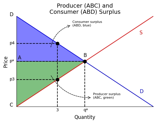
But for some of the early units, the cost of production was lower than p*. For example, if we assume q* is more than 3, the 3rd unit sold cost p3 < p*. So the firm made a profit of p* - p3 > 0 on that unit. (Recall that the supply curve includes the opportunity cost of capital, including the equity holders’ capital. So we are talking about economic profit.) That is true for all the units up until q* (which costs exactly p* to make). So the producer’s full profit is the triangle ABC. We call this triangle the producer surplus. It captures the producers’ gains from trade in a free market.
Turning our attention to consumers, we see that some consumer was willing to pay p4 > p* for that unit. If we apply the same logic we used for producers, that means that consumers earned a sort of profit on that too: consumers got a thing worth p6 for just p*. That is true for each unit up until q*, which is worth exactly p* to consumers. So the consumer’s gain from trade is the triangle ABD. We call this the consumer surplus.
The total gains from trade, across producers and consumers, is equal to the sum of producer surplus and consumer surplus. This is also called total surplus or social surplus.
Efficiency
To determine whether markets are efficient, we need to define efficiency. We will use our understanding of surplus to contrast different definitions of efficiency.
Efficiency is a term used to describe an allocation of resources amongst people, including producers and consumers. It is easier to understand efficiency if you focus on 1 market for 1 good, and hold the allocations of all other resources the same. Then we can think of an allocation as a combination of quantity and price for a good in one market.
Economics typically uses either of two definitions for efficiency. One definition of efficiency asks if a particular allocation of goods can be changed so that at least one person is better off, and no one is worse off. If an allocation meets this condition, then we say the allocation is Pareto efficient relative to the first.2
We can illustrate a Pareto improvement with the figure below. If we choose a quantity and price of (q1, p1), to the left of the intersection of demand and supply, consumers are willing to pay more (p2 > p1) for an extra unit than it costs producers to supply that unit (p0 < p1). If we choose another allocation at (q3, p1) that entails higher quantity at the same price, producers will be willing to supply that amount, since price p1 is greater than their cost of production p3. Moreover, consumers will buy the extra goods since their willingness to pay p4 is greater than the price p1. We can verify that both groups are strictly better off by looking at the consumer and producer surplus. Both grow from the dark blue and dark green regions to the area covered by the dark and light blue and green regions, respectively. The intuition here is that the price remained the same, so both producers and consumers got as beneficial a deal as before, but quantity increased, meaning there were more deals for each side.

Query: Suppose we started with an allocation of (q1,p0) and assume each consumer buys just 1 unit of the good apiece. Show that we could not change allocation to make everyone better off. Hint: show that at least some consumers must lose with any other allocation with greater quantity that producers would want to supply.
The second common definition of efficiency is a bit more relaxed than the first. Under this definition, one allocation (price-quantity combination) is better than a second allocation, if it provides more net benefit to consumers and producers than another. There is no requirement that no one loses under the second allocation. Instead, we ask whether the winners make enough extra that they can fully compensate the losers. This definition of efficiency is called Kaldor-Hicks efficiency.3 Indeed, if we were to couple a Kaldor-Hicks efficient allocation with transfers from the winners of the new allocation that compensate the losers from the new allocation, the combination of the new allocation and those transfers are a third allocation that is Pareto efficient relative to the original allocation. It is this reason that we say that Kaldor-Hicks is a more relaxed standard relative to Pareto efficiency: you need to add something to the Kaldor Hicks allocation to make it Pareto efficient. And a Pareto efficient allocation is always Kaldor Hicks efficient.
The figure below illustrates a Kaldor Hicks efficient allocation. We start with a different allocation than before: (q1, p0) rather than (q1, p1), where p1 > p0. Our second allocation is (q3, p1) as before. Going from (q1, p0) to (q3, p1) increases the sum of consumer and producer surplus. So it is Kaldor Hicks efficient: the total gains from trade are larger under the second allocation. But clearly some consumers lose: any consumers who purchased the first q3 units have to pay a higher price under the second allocation. So this second allocation is not a Pareto improvement.

So which definition of efficiency will I use in this course? In the main, we will use the second one: Kaldor Hicks. The reason is that we will not be concerned with distribution of gains and losses as much as Pareto efficiency is. Sometimes we may talk about who gains and loses with different allocation rules or regulations. But we’ll flag those in the context of discussions about Kaldor Hicks efficiency.4
When and why is a market efficient?
Now we can address the question: When and why is a market efficient? Let’s start with when. Here is what we are going to assume:
Property rights over the good are well defined and enforced.
There are no transaction costs.
The demand curve reflects social marginal value.
The supply curve reflects social marginal cost.
Producers are competitive, i.e., cannot collude to raise the market price.
There is no relevant asymmetric information.
The goods in question are private goods, i.e., they are rivalrous and excludable.
There are no price regulations or taxes, so that the market equilibrium is the intersection of the demand and supply curves.
Under these assumptions, markets are efficient. Before we explain each assumption and why it is important, let’s use what we have learned about surpluses and the definition of efficiency to sketch the argument for why markets are efficient.
The figure below illustrates the market equilibrium in assumption #8 (intersection of supply and demand) and highlights the consumer and producer surplus under that equilibrium. We can demonstrate that the market is efficient by showing that there is no way to increase the total surplus (i.e., consumer surplus plus producer surplus).

Let’s initially hold q at or equal to q*. To increase consumer surplus, but keep quantity below q*, we would have to lower price below p*. (We cannot shift the demand curve, otherwise assumption #3 is violated.) But if we lower price, then producers would not want to produce q* because q* costs p* to make and producers will not produce an additional unit if they lose profit doing so. As a result producer surplus falls, and the fall in producer surplus exceeds the increase in consumer surplus. Conversely, to increase producer surplus, but keep quantity below q*, we have to increase price (analogously because we cannot shift the supply curve without violating #4). But then consumers would want fewer units. So consumer surplus would fall, and by more than producer surplus would rise. So, given our demand and supply curve, we cannot increase surplus in the space between them and keep quantity below q* above the surplus provided by the market equilibrium.
What if we allow quantity to rise above q*? Markets remain the best one can do. To the right of q*, the supply curve is above the demand curve. This means each additional unit costs more to produce than that unit is valued by potential consumers. Such units generate social losses instead of surplus. So increasing quantity cannot ever increase surplus, and thus cannot be more efficient than the market equilibrium.
Query. Note that what we have said does not mean that there are no other allocations that produce the same surplus as a market equilibrium. Ask your favorite LLM about, e.g., perfect price discrimination. Ask how it can lead to the same social surplus as a competitive market, but even higher producer surplus than in the figure above. Note, however, that it involves a violation of condition #5, which is that markets are competitive.
When and why do markets sometimes fail?
Markets fail, intuitively, when the assumptions required for markets to be efficient do not hold. So let’s walk through each assumption and understand what it means. (We will explore the violation of several assumptions in more detail in subsequent lectures.)
Property rights over the good are well defined and enforced.
There are no transaction costs.
If you've heard of the Coase Theorem, these two assumptions should be familiar. The two assumptions are required for any allocation of property rights (which is the right to engage in some action) is efficient. Well, you can also have property rights that include possession of goods. Given that, the Coase Theorem applies to trade in goods and not just rights to take actions (besides possession of goods).
The reason we want property rights to be well defined and enforced is that we need to stop theft. With theft, a producer cannot ensure that it will receive p* for a unit of its good. A thief takes it for p = 0. In that case we would have 0 production and excess demand!
The reason we want no transaction costs is that they operate like taxes. And taxes, as we shall see, cause a wedge between the price a consumer pays and the price a producer receives. This causes quantity to fall below q*. The thing that makes transaction cost worse than taxes is that the expenses on transaction cost do not become revenue for the government. Instead, they are partly wasted on things (paperwork, etc.) that no one intrinsically values.
One of the purposes of property law, and basic state capacity, is to ensure that assumption #1, that property rights are well defined and enforced, is met.
The private demand curve reflects social marginal value.
The private supply curve reflects social marginal cost.
A private demand curve and a private supply curve mean the demand and supply curve of those individuals and companies actually participating in the market for a good. The private demand curve reflects the private marginal value (or willingness to pay) of individuals who are consumers in the relevant market. The private supply curve reflects the private marginal costs of producers who are supplying the good to a market. The social marginal value is the marginal value to all people – not just the consumers – from consumption of a unit of the good in question. Likewise, the social marginal cost is the marginal cost of production accounting for costs not just to producers, but all people in society, from production of a unit of the good.
Usually, these two assumptions are intended to rule out externalities. An externality is an external effect from the action of one person on another person. The externality is a negative externality if the person at the receiving end of the external effect has a property right to be free from that external effect. For example, if I have a right for my car not to be damaged by you, and you crash into my car, then you have had a negative externality on me. (Conversely, a positive externality is if I have a right and you increase the value of my right.)
The externality may flow from consumption or from production. For example, my consumption of a car may cause a risk to your health due to pollution from my car. This would mean that the private demand curve for cars, which reflects private marginal values of consumers of cars, is lower than the social marginal value of consumption, which also captures the health costs to people who do not own cars from the driving of cars by car owners. Likewise, the manufacture of cars may cause pollution that affects individuals other other than the producers. This would not be captured by the supply curve, which measures the marginal cost of producers, but would be included in the social marginal cost of production. In this case, the private supply curve would be lower than social marginal cost.
The market equilibrium sets price and quantity, i.e., the allocation of resources, at the intersection of the private demand and supply curve. But social surplus is maximized when at the allocation given by the intersection of the social marginal value curve (i.e., the social demand curve) and the social marginal cost curve (i.e., the social supply curve). If there are no externalities, the private social demand curve, and the private and social supply curve are the same. So the surplus from a private market is equal to the maximum social surplus possible.
One of the purposes of tort law is to ensure that private supply and demand curves internalized externalities and thus equal the social marginal cost and marginal social value curves. I.e., tort law helps ensure assumptions #3 and 4 are met.
Producers are competitive, i.e., cannot collude to raise the market price p*.
Competition ensures that the market price is p*. If one producer raises its price above p*, other producers undercut that producer and the first producer loses its sales. Consumers are always able to buy the good at p*.
If producers could collude, they could raise the price without being undercut by other producers. This strategy would lower the quantity consumers purchase (because the demand curve slopes down). But it could, if the price was set just right, raise the producer’s surplus. But, as we shall see, the higher producer surplus would come at the expense of consumer surplus and total surplus. That would make the market inefficient because we have shown total surplus is greatest when price is set by a competitive market (and all other assumptions besides #5 hold).
Ensuring this assumption holds is one of the goals of antitrust policy, which targets producer collusion.
There is no relevant asymmetric information.
Asymmetric information means that there is a difference between the relevant information that one party to a trade has and the other party to the trade. Note that asymmetric information only matters if the information is relevant. If the business does not know the consumer’s banking password, that does not prevent markets from being efficient.
Let me give you a somewhat advanced example of asymmetric information that does affect the efficiency of markets. (My example is borrowed from Einav & Finkelstein 2011). Consider the market for health insurance. An important feature of this market is that different people have different health conditions, so may require different levels of medical expenditures. This means the cost to a health insurance company (the producer) of providing insurance for one consumer may be different than for another consumer. In other words, the marginal cost of production is not the same for all insurance consumers. This contrasts with the case of, e.g., pants. The cost of production for pants (of a given size and design) does not depend on who wears them.
In the figure below, we plot the demand and supply curves for 1 year health insurance contracts with a fixed coverage (e.g., $1000 deductible, 10% copays, $8000 annual out-of-pocket cap, and no annual coverage cap). Each consumer purchases at most 1 contract. We assume that individuals with a higher level of expected medical expenditures have a higher willingness to pay for health insurance, and draw a corresponding downward sloping demand curve for health insurance consumers. To plot the supply curve we need to account for the fact that the marginal cost of coverage varies across individuals and the way insurance is priced. In particular, the marginal cost of insurance is higher for those with higher expected expenditures, i.e., for those with higher value from insurance. This means that, if companies know each individual’s cost and the company can charge different prices to each individual consumer, then the (marginal cost) supply curve is also downward sloping, a change from how we previously drew the supply curve. If the supply curve is flatter than the demand curve and intersects it once, then the market produces an efficient outcome (p*, q*) where quantity is given by the intersection of the demand curve and the (marginal cost) supply curve. The market is a bit unusual, however, because, recall, each individual is charged a different price for insurance. By contrast, in more usual markets, the price of a good is the same for each person.

Now let’s introduce information asymmetry. Specifically, we will assume that each consumer knows her own expected medical expenditures, but that the insurance company does not know those expected costs. Instead, all a company knows is the average cost of covering a group (or “pool” of consumers) that purchases its insurance contract. As a result, the insurance company has no choice but to charge each consumer the same price. What is that price? Instead of charging each consumer a price equal to the marginal cost of covering that consumer, a company would charge each consumer the average cost of all consumers that purchase insurance from the company.5
This means that the supply curve, under information asymmetry, is equal to the average cost curve, rather than the marginal cost curve. Because the average cost of a group of consumers is the average of marginal costs of all consumers in the group and consumers with the greatest demand have the greatest marginal cost, the average cost curve will be decreasing in quantity of contracts produced. Specifically, the average cost curve will be the same as marginal cost for the first contract, but then lie above the marginal cost curve for each subsequent contract produced. This means that, in our figure, the average cost curve intersects the demand curve to the left of where the marginal cost curve does.
Under information asymmetry, the equilibrium output of insurance will be where the demand curve intersects the average cost curve (p’, q’), rather than where it intersects the marginal cost curve. Since the average cost intersection is to the left of the marginal cost intersection, the total output under information asymmetry will be lower than output under no asymmetry. Because the efficient output is given by the marginal cost intersection, we may conclude that information asymmetry causes insurance companies to sell too little insurance to consumers. This is a species of what is called adverse selection because the people who tend to still buy insurance are selected (by the higher price of insurance) to be higher cost individuals.
This is just one example–albeit a common example–of how information asymmetry can cause market failure. It is unlikely that, in an introductory law and economics or microeconomics course, we will cover information asymmetries at depth. However, one can explore this and other complications from information in an advanced course or an information economics course.
Query (hard!): Try to use simple supply and demand to model the demand for criminal defense when different clients have different costs to defend, and the criminal defendant knows more than her lawyer. Use the model of Einav & Finkelstein (2011) to explain why there might be inadequate consumption of legal services if lawyers had to charge all clients the same amount. If lawyers could charge by the hour, would that solve the problem?
Various areas of law address information asymmetries. Consumer protection law addresses situations where the producer has more information than the consumer. Insurance and healthcare law has a number of provisions, including insurance mandates and subsidies, that attempt to address adverse selection.
The goods in question are private goods, i.e., they are rivalrous and excludable.
Economics classifies goods into four categories based on two factors: whether a good is rivalrous and whether it is excludable. A good is rivalrous if my consumption of it prevents you from consuming it. One example is a cookie: if I eat it, you cannot also eat it. A good is excludable if the producer of the good can stop people from consuming it. An example is a TV: Best Buy can make sure you do not take a TV, until you pay Best Buy its price for that TV.
In the figure below, reproduced from Jones & Vollrath (2013), you can see examples of goods that are different combinations of rivalrous and excludable. Goods that are both rivalrous and excludable are called private goods. Goods that are neither rivalrous nor excludable are called public goods. Goods that are rivalrous, but not excludable are called common-pool goods. And goods that are excludable, but not rivalrous are called club goods (or artificially scarce goods).

If a good is non-excludable, its producer cannot stop people from consuming it without paying. Therefore, the producer cannot be sure it will recoup the costs it incurred to produce the non-excludable good. Knowing this, the producers will not produce adequate amounts of the non-excludable in the first place. I.e., the non-excludable good will tend to be undersupplied. One implication is that markets tend to be inefficient because they do not supply an adequate amount of public goods.
Even if the non-excludable good already exists in nature, i.e, is already produced in adequate quantity, it will tend to be over consumed because the market cannot impose a price for its consumption. Individuals will take it without paying, and impose a social cost equal to the value that other consumers might have gotten from the good if they had consumed it. This problem, which afflicts common pool goods is called tragedy of the commons.
The last category of goods ruled out by assumption assumption #7 is club goods. These goods are non-rivalrous, but can artificially be made excludable. For example, a movie theater owner might only show a movie inside an auditorium and charge people to enter the auditorium. (But consumption by one person in the theater does not affect the consumption of another person in the theater.)
There are at least two reasons why markets for club goods are inefficient. First, making club goods excludable often entail large fixed costs. These costs lead to (local) monopolies being more efficient producers. (Why pay a fixed cost twice?) But monopolies tend to raise price the competitive equilibrium price, raising producer surplus at the expense of total surplus. Second, the cost of exclusion is different than the cost of producing club goods. As a result, the price in club goods markets tends to be above the marginal cost of production. This leads to the under provision of club goods.
The problem of public goods is addressed not by regulation but by spending: one justification for government spending on or production of public goods is that private markets undersupply them. The problem of common pool resources is often addressed by environmental regulations that limit the quantity of consumption (e.g., fishing). Finally, club goods implicate both antitrust law, which scrutinizes monopoly producers of club goods, and local government law, because local governments often provide benefits only to local taxpayers such as access to local parks.
There are no price regulations or taxes, so that the market equilibrium is the intersection of the demand and supply curves.
The last, but not least important, assumption required for markets to be efficient is that the government does not impose taxes or regulations that prevent markets from setting a price p* that equalizes supply and demand. If the government sets price floors above p* or price caps below p*, then obviously the market cannot allocate resources using p*. That means that there will either be excess supply or excess demand, respectively. Taxes are not a direct constraint on prices like price controls. However, they do create a wedge wherein consumers have to pay a higher price than producers receive. This causes market output to be lower than optimal. There will be units that are efficient to trade because marginal value to consumers will be above marginal cost to producers, but the gap is smaller than the tax and so trade does not happen.
This assumption directly implicates law, not because law tries to ensure markets are efficient, but because law is the cause of market inefficiency.
References
Einav, L., & Finkelstein, A. (2011). Selection in Insurance Markets: Theory and Empirics in Pictures. Journal of Economic Perspectives, 25(1), 115-138. https://doi.org/10.1257/jep.25.1.115
Jones, C. I., & Vollrath, D. (2013). Introduction to Economic Growth (3rd ed.): W.W. Norton.
You might wonder why the notion of economic profit does not align with the common sense notion of profit, which matches the accounting definition. The common sense notion thinks of profit as something earned by owners, and owners are the equity holders. It would make no sense, then, to subtract from the dividends paid to owners the amount they could have earned in another investment: the latter amount still goes in owners’ pockets.
But there are two reasons to focus on economic profits rather than accounting profit. First, people have trouble thinking of a firm as an actor that is different from the firm’s owner, typically the firm’s equity holder. However, large firms have managers that are separate from owners and that control the firm. Moreover, sometimes those managers are beholden to their own interests or the interests of debt holders, not those of equity holders. I.e., shareholders do not always control the firm. Second, the extra amount that an equity owner earned from a firm should not include the amount she could have earned in any other investment, i.e., the opportunity costs of financial capital. That would overcount the return to investing in a firm. So we should consider as profit the dividends paid to firm owners minus the opportunity cost of firm owners’ capital investment. This is the same as economic profit.
ChatGPT on Vilfredo Pareto, the inventor of Pareto efficiency: “Pareto efficiency is named after Vilfredo Pareto, an Italian economist and sociologist. Born July 15, 1848, in Paris, Pareto was the son of an exiled Italian nobleman. He studied engineering at the Polytechnic University of Turin and initially worked as a civil engineer and manager. His interest in economics and social theory emerged later in life, leading him to academia. Pareto became a professor at the University of Lausanne in Switzerland, where he developed theories on income distribution and social choice. His most famous contribution is the Pareto principle (80/20 rule) and the concept of Pareto efficiency, foundational in welfare economics. Pareto also studied societal elites and cycles, blending economics with sociology. He died on August 19, 1923, in Celigny, Switzerland. Despite controversy around some of his sociological views, his economic theories remain highly influential.”
ChatGPT on the architects of Kaldor Hicks efficiency: “The concept of Kaldor-Hicks efficiency is named after Nicholas Kaldor and John Hicks, two influential 20th-century economists. Here's a brief description of each:
Nicholas Kaldor (1908–1986):
A Hungarian-British economist, Kaldor was a key figure in post-Keynesian economics. He contributed to theories of growth, income distribution, and welfare economics. Kaldor is best known for his work on the trade-off between efficiency and equity, the development of the "Kaldor facts" about economic growth, and his input in designing policies for full employment and industrial development.
John Hicks (1904–1989):
A British economist and Nobel laureate, Hicks is celebrated for his work in microeconomics and welfare theory. He introduced the IS-LM model and contributed to consumer theory with the Hicksian demand function. Hicks played a pivotal role in developing the compensation principle, a cornerstone of Kaldor-Hicks efficiency, linking economic efficiency with potential wealth redistribution.”
When I say that Pareto efficiency places more emphasis on distribution, you should not interpret that as greater emphasis on progressive distribution. Under Pareto efficiency, it could be possible that a second allocation is not Pareto efficient because it hurts rich people rather than poor people, I.e., entails a regressive redistribution. The Pareto criterion does not distinguish between progressive and regressive re-distributions: it penalizes both.
By the way, you could get the same result if you assumed that a government regulation required that the insurance company charge the same price for every consumer, even if the company knows which consumers cost more and cost less. (Such a regulation is called a community rating regulation. It contrasts with experience rating, which means charging a different price to consumers based on the company's assessment of each consumer’s expected medical costs.) Under a common price regulation, the company would charge average cost if there were a competitive market in insurance because that would allow the company to break even.