

Market failures: Price regulations and taxes

[This essay is intended for students in my law and economics and my microeconomics class (for law students). Read this essay one time through, ignoring the queries that are interspersed. Go back to the queries after you feel you have understood the essay. The queries test whether you have understood enough to develop a richer understanding of the topic of the essay (price regulations and taxes). These instructions will also apply to future essays.
I have bolded certain words. These are terms that you should know going forward. If you do not understand them, ask your favorite foundational AI model about them.
I will post the python notebook that generates all the figures in this essay in case you are interested in reproducing them.]
In the last essay, we discussed the assumptions under which a market equilibrium would be (socially) efficient. One of these assumptions was that there are no price regulations or taxes. In this essay I explore why price regulations and taxes lead markets to have inefficient allocations.
Before I begin, I want to frame the problem and I want to comment on the broader relevance of the logic and examples I provide below.
I framed the problem of price regulation and taxes as a market failure. And many people respond to market failures by calling for government action. I recommend being more cautious. Price regulations and taxes are themselves government actions. So this is a market failure caused by government policy. Perhaps government action is also the solution. But the correct government action may be to deregulate: eliminate price controls or taxes. The solution is not necessarily for the government to take additional actions to redistribute products or impose different price controls. As such, it may be better to frame price regulations and taxes as government failures rather than market failure. Markets may have worked just fine if the government had not intervened.
While we will speak to price regulation and taxes, the analysis below is a bit more general. Readers should be able to use similar logic to understand why quantity regulation or subsidies can also lead to market failures.
With these prefatory comments out of the way, let’s analyze price regulations.
Price regulation
In order to isolate the effects of price regulation on markets, we will assume that all the other assumptions required for markets to yield efficient results continue to hold. Foremost among these will be that private demand and supply curves reflect social value and costs, respectively. People will often object to arguments that price controls and taxes are inefficient by arguing that we need these interventions to stop externalities. That may be correct, but price regulations and taxes are often imposed even when there are no externalities. Here we analyze a situation in which there are no externalities. We will examine the case where private and social demand and supply diverge in another essay.
Let’s start with a properly functioning market, as in the figure below. We have aggregate demand and supply curves that intersect at (q*,p*). There are no price regulations, and all the other assumptions required for efficient markets as assumed to hold. So this (q*,p*) is an efficient allocation.
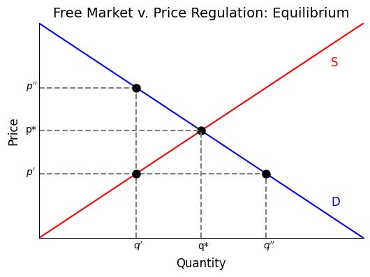
Suppose we impose a price control requiring price to be p’, below p*? The demand curve tells us that the quantity demanded would be q’’, which is greater than q*. But the supply curve says that the quantity firms would supply would only be q’, lower than q*. Because quantity supply is also less than quantity demanded, there would be excess demand.
The amount of goods exchanged is the lower of the quantity supplied or demanded. This is because US contract and property law, in general, ensure that markets only trigger voluntary trades.1 If a firm does not want to supply a good that consumers want, they can’t be forced to do so. Likewise, if a consumer does not want to buy a good that the firm produces, she cannot be forced to buy the good. So the price control at p’ causes the equilibrium quantity to be q’, which is lower than q’’.
How can we show that this result is inefficient? We will use the Kaldor Hicks criterion for efficiency and look at total surplus without and with price controls. In the figure below, we re-draw market equilibrium with and without the price control, but then label parts of the consumer surplus into areas A, B, and C, and part of the producer surplus into areas D, E, and F. If there were no price controls, the efficient allocation would be (q*,p*). This means total consumer surplus is A + B + C, the area below the demand curve (consumers’ valuations) but above the price line. The total producer surplus is D + E + F, the areas below the price line but above the supply curve (firms’ costs).
If the price control sets price at exactly p’, consumer surplus depends on who buys the good. There is a wide range and how much consumers who would buy the good value the good at. Some value the good at p’’’, which is where the demand curve intersects the y-axis, others value it at just p’, and many in between. To be conservative, let's assume that amongst all these consumers, it is the ones who value the good the highest that will purchase the good. This assumption will cause us to underestimate the inefficiency of price controls, but even this underestimate is enough to help clarify why price controls cause social loss.
Under this assumption, the consumers who buy the good under our price control are those who value the good greater than p’’, which is where q’ intersects the demand curve. Consumers who value the good more than p’’ are those who value it the most. These consumers were willing to pay at least p’’, but only had to pay p’ for the good. That means the consumer surplus is A + B + D. The producer surplus is simply F, the area below p’ but above the supply curve. No areas to the right of q’ are part of the surplus calculation because that is the maximum quantity of voluntary transactions.

To compute the social loss, or the level of inefficiency, with price controls, let’s list the total surplus with and without price controls, and determine the difference. The table below lists the consumer surplus, producer surplus, total surplus (sum of CS and PS) for the market without price controls and the market with a price control at p’. The bottom row compares the total surplus with the price control against the surplus without it. We can think of this as a social loss from price control, because it is opportunities for gainful trade that were eliminated by the price control. Economists also call such social loss “deadweight loss”.

The table reveals that the social loss is C + E, the area to the right of q’ where the demand curve is higher than the supply curve. It is the area to the right of q’ because that is the maximum amount producers voluntarily supply under the price control p’. It is the area where demand is greater than supply because those are the only trades that would occur in a market free of price controls. (To the right of q*, the cost of goods is greater than the willingness of consumers to pay for them, so no voluntary trades occur there.)
Query. If, instead of a price control at p’, the government set a price floor at p’, there would be no inefficiency in the market. (A price floor at p’ allows consumers to buy at a price above p’. Prices below p’ are prohibited.) Explain why this claim is true.
Query. A price ceiling at p’ has the same deadweight loss as a price control at p’. (A price ceiling says the maximum price at which a good can be sold is p’. Prices below p’ are permitted.)
Query. If we do not assume that consumers who value the goods the most are the ones that purchase the q’ goods sold, what happens to consumer surplus? What happens to total surplus and thus welfare loss under price controls?
Query. Suppose a lottery is used to allocate q’ among the set of consumers willing to pay at least p’. Moreover, these consumers can re-sell the good to any consumers who value the good without any transaction costs. How does that affect consumer surplus? Who gets that surplus? How does it affect total surplus and efficiency?
Instead of a price control at p’, suppose the price control were set at p’’ above p*. There would now be excess supply, because firms would want to supply q’’, but consumers would only want q’. Roles would be reversed. Because quantity demand is lower than quantity supply, quantity demand now determines the quantity transacted.

We can use the same diagram above to determine the welfare loss with a higher price control at p’’. Consumer and producer surplus in the no price control scenario is the same as before. But with price control at p’’, consumer surplus falls to A. The reason is that the price is higher, now p’’, and A is the area below the demand curve but above the new price.
What about producer surplus? Let’s assume that it is the lowest cost producers who supply the q’ goods that consumers demand. (This is analogous to the assumption, when the price control was at p’, that only the highest value consumers would buy the q’ goods that producers supply.) This assumption ensures that the welfare loss we are about to calculate is actually an underestimate of the welfare loss under price controls. Under this assumption, producer surplus is B + D + F. That is the area below p’’ that is above the supply curve for the lowest cost producers.
The total surplus is A + B + D + F, as before, though the higher price control gives producers more of the total surplus.
Query. If we do not assume that producers who have the lowest marginal cost of production are the ones who supply the q’ goods consumers purchase, what happens to producer surplus? What happens to total surplus and thus social loss from price controls?
Comparing this to surplus without price controls shows that the welfare loss with price controls is C + E. Qualitatively, this is the same as before. (Actually it is quantitatively the same because we set p’ and p’’ to be the same in both cases. But that may not be the case in future examples you see.) Whether regulation sets a low price or a high price, price regulation will reduce the amount of trade. The welfare loss is the product of losing out on the gains from trades that do not occur because of price controls.
Query. Suppose the government not only regulates that price be p’’ but randomly picks firms to supply the good, until q’ output is produced. However, the chosen firms can buy the amount of the good that they are required to produce by the government from other firms instead of producing it themselves. Assume there are no transaction costs. What is producer surplus and who obtains it? How does this affect efficiency? Can you draw an analogy between this problem and markets for tradable emissions permits? What happens in this problem if there are high transaction costs, and what does that tell you about the importance of transaction costs? Bonus: Relate this all to the Coase Theorem.
Taxes
Let’s turn our attention from price controls to taxes. While price controls tell people the price they must transact at, taxes tell people what price they have to pay to transact. There is no direct regulation of the price of a transaction, but the requirement to pay a tax will limit the prices at which trades are possible. Taxes also allow the government to participate in—i.e., take a part of—the gains from trade. However, that extraction comes at a cost: taxes also impose a deadweight loss.
Start again with our free market diagram, where the efficient allocation is (q*,p*). Suppose we impose a tax of t, i.e., each time a consumer wants to buy a product at price p, it has to pay a tax t to the government. This is not a proportional tax, e.g., pay t% of the price or a total of (1+t)p. It is a fixed tax meaning the total price is p+t.

How much will consumers purchase from suppliers? To find the answer, consider what price would clear the market when the producer has to pay a tax of t, i.e., what price (before taxes) would cause consumer demand to equal producer supply. The amount that determines how much the producer supplies is the amount it pockets from the transaction. This is p, not p+t, because the t part goes to the government. So the price the producer quotes is what drives the quantity it supplies. The amount that determines how much the consumer wants to buy, however, is p+t. Why? If the producer receives p, and the government gets t, then the consumer must pay p+t.2 So, to clear the market, we need to find a price p where the quantity supplied at p is equal to the quantity demanded at p+t. That quantity is easy to find: it is the quantity where the vertical distance from the demand curve to the supply curve is equal to t. I labeled that q’ on the figure above. From that quantity, I can see that the price p’ generates that quantity of supply. I can also see that the price p’’=p’+t generates that quantity of demand. And clearly the vertical gap between p’ and p’’ is t.
Now we can calculate the welfare effects of taxes, i.e., the social loss associated with taxes. The figure below draws the same graph above, but tags different areas of the graph with letters, A through F so that we can calculate the social surplus before and after taxes.

The surplus before taxes is the same as in the case without price regulation that we examined earlier. The surplus after taxes, however, is a bit different than under price controls. The reason is that taxes allow the government to seize some of the gains from trade. Because the price received by the producer is p’, that means the producer surplus is F. The consumer faces a price of p’’ = p’+t, so the consumer surplus is A. The total taxes collected by the government is t x q’, i.e., B + D. In the price regulation example where the price was set to p’ and somehow only the highest value consumers still obtained the good, this surplus (B + D) went to the consumers. Now it is collected by the government via tax revenue.
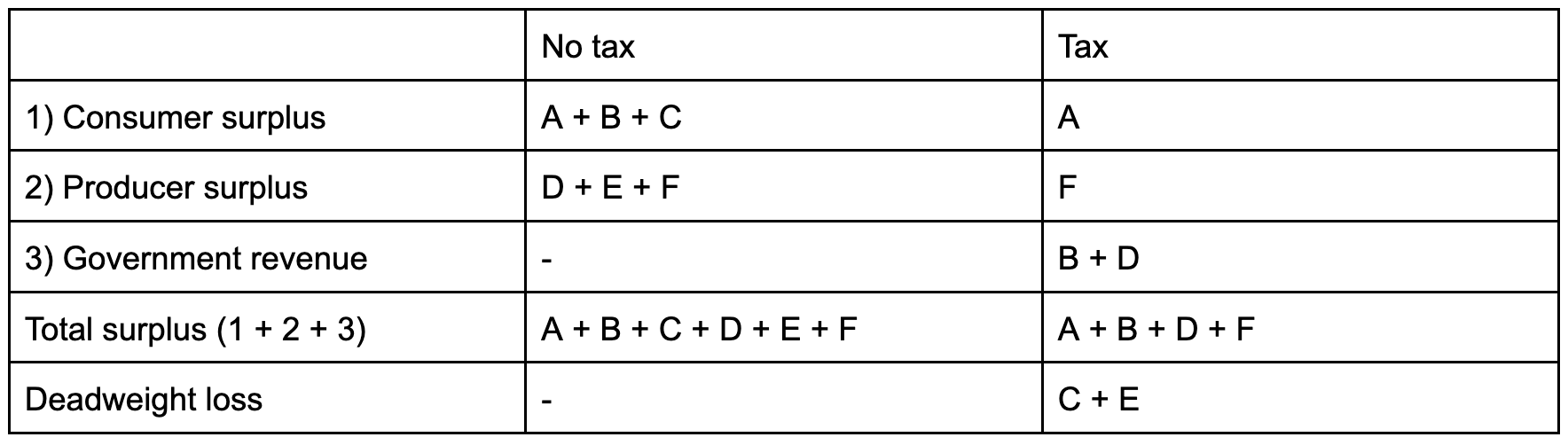
The table above lists total surplus with and without a tax. It differs from the tables in the price control section because it has an extra row for the government’s revenue collection. However, total surplus includes the government. So total surplus with taxes is A + B + D + F. (While this is the same under the p’ price control example above, that is strictly true only if both cases have the same demand and supply curves and the p’ here is the same as the p’ earlier.) Comparing this surplus to that with no tax, we see that the social loss is C + E. Live price controls, taxes limit trade and thus gains from trade. For trades above q’, the difference between what consumers are willing to pay and what producers get is not enough to cover t, the tax that the government imposes on each transaction.
An implicit assumption in our welfare calculation is that the social value of government revenue from taxes is equal to the quantity of that revenue, i.e., B + D. That is not obviously true. If the government uses that money to build something consumers and producers value more than B + D, e.g., roads or national defense or social insurance, then social welfare with taxes is greater than A + B + D + F. Conversely, if the government wastes that money, then the welfare value is less than B + D, and social welfare with taxes is less than A + B + D + F. Economists call the value of $1 of spending by the government the government multiplier. When that multiplier is greater than $1, that means society gets more than $1 of value from $1 of government spending. The multiplier is less than one if society gets less than $1 of value from $1 of government spending.
Tax incidence
Earlier I said that a legal requirement that the producer write the check for taxes to the government does not mean that the producer bears the burden of the tax. More generally, knowing who is nominally paying the taxes on a transaction, producers or consumers, does not determine who actually bears the burden of the tax. Who bears the economic burden of a tax is called the incidence of a tax. And the burden or incidence of the tax depends on the relative slopes of the demand and supply curves. Because different goods have different units for quantities, we use elasticities to convert slopes of demand and supply curves for different goods all into percentage units. So, another way to state my point is that the incidence of taxes depends on the relative elasticities of demand and supply curves for a good.
In particular, the party that has the relatively more inelastic supply or demand curve will bear the burden of a tax. To see this, start with the black supply and demand curves below. When a tax of t is imposed, we can see that the consumers hand over B to the government, while the producers hand over D. The consumers’ share of total taxes paid, is the surplus they sacrifice when a tax is imposed. Since total tax revenue is B + D, the consumer share is B / (B+D). Likewise, the producers’ share is D / (B+D).

Now suppose we make the producer’s supply curve completely elastic, i.e., flat, as in the blue lines.3 Now, when we impose the same tax, the price p* the supplier receives before and after the tax is the same, but the price that the consumer pays is much higher, p* + t rather than p’ + t. The suppliers’ surplus doesn’t change (it is 0 before and after). The government’s revenue now comes entirely from the consumer: it is B = q’’ x t. So the consumer bears all the tax. This is apparent from the fractions we use to calculate the incidence of taxation. When supply is perfectly elastic, D is 0. So the consumer share is B / (B+D) = B / B = 1. Meanwhile, the producer share is D / (D + B) = 0 / B = 0. The consumer bears the full burden.
Query. Do the same exercise except go from the black lines to one where the consumer is perfectly elastic and the producer’s supply curve does not change.
More generally, the formula for computing the incidence of a tax is
Change in consumer price = t x Es / (Es + |Ed|)
Change in producer price = t x -|Ed| / (Es + |Ed|)
where Es is the price elasticity of supply and Ed is the price elasticity of demand. Here incidence is calculated as the increase in consumer price (relative to no tax) and a decrease in producer price. That is reasonable because you just have to multiply by the quantity transacted to get tax revenue.
Aside. You can derive this formula using some calculus. Remember that markets set prices to ensure demand equals supply. When there is a tax of t, that means D(p+t) = S(p), where S is not quantity supplied and D is quantity demanded. This means S(p) - D(p+t) = 0. Take the derivative of both sides with respect to the tax: dS/dp dp/dt - dD/dp - dD/dp dp/dt = 0. Solve for dp/dt to get the change in price for suppliers: dp/dt = dD/dp / (dS/dp - dD/dp). To convert the right hand side to elasticities, multiply the numerator and denominator by the S/p or D/p (they are the same since S = D in a market). To get the total change in price, multiply both sides by the amount of the tax. Then To get the elasticity, multiply both sides by T.
The formula for incidence is very useful. It not only tells you who bears the burden of a tax, but also the gains from a subsidy or the burden of a regulation that increases the cost of consumers or producers. For example, if the government gives you a subsidy to go to college, colleges will extract some of the value from that subsidy. If the government imposes a requirement for a company to provide a more generous warranty for its products, some of the cost of that warranty will fall on the company’s customers.
This is not always the case. There may be cases where the law bars trades parties want to have. Indeed, the price regulation we are examining does just that. Firms and consumers who want to transact at some price above p’ cannot do so. Indeed, there may be cases where the law requires trades that firms and consumers would prefer not to undertake because there is no surplus. An example is when the government requires producers to supply a product feature that consumers do not want. An example is regulations that require producers to provide warranties that consumers do not want either because the cost of the warranty is too high or the value of the warranty to consumers is too low. But the general rule is that US law tends not to require involuntary trades.
You might be confused and ask: didn’t you say that the producer pays the tax? My superficial answer is yes, but the producer has to get the money to pay the tax from someone, and that is the consumer. The producer only has to pay the tax on sales it makes, not sales it does not make. My deeper answer will come later, when I explain that, regardless of who formally has to send a check to the government, the producer and consumer actually share the burden from the tax.
Recall that elastic supply does mean that the slope of supply is very steep. The reason is that the supply curve compares price on the y axis to quantity on the x, so the slope is change price over change in quantity. But the price elasticity of supply is % change in quantity over % change in price, the inverse. So a high elasticity means a low slope for supply.