[This essay is intended for students in my law and economics and my microeconomics class (for law students). Read this essay one time through, ignoring the queries that are interspersed. Go back to the queries after you feel you have understood the essay. The queries test whether you have understood enough to develop a richer understanding of the topic of the essay (deriving a demand curve from preferences and a budget constraint). These instructions will also apply to future essays.
I have bolded certain words. These are terms that you should know going forward. If you do not understand them, ask your favorite foundational AI model about them.
I will post the python notebook that generates all the figures in this essay in case you are interested in reproducing them.]
Thanks for reading Research Notes! Subscribe for free to receive new posts and support my work.
Today, we are going to derive a demand curve. Looking forward, we're going to need a demand curve to figure out how much consumers are willing to pay for a particular good. When we combine that with the supply curve (which will drive in a future essay), we will get the price that will ensure that the quantity that consumers demand is equal to the quantity that producers supply. Moreover, that quantity will be the output that we will see from a market.
But it all starts with a demand curve. A demand curve tells us how much consumers are willing to pay (denominated in dollars) for a particular good. If consumers do not demand a good, there is no market because, without paying customers, there's no reason producers will pay the cost of producing a good.
An important feature of demand curves is that, with very few exceptions, they slope downwards. I.e., if the price of a good rises, people want less of it. This is such a regular feature of our world that economists call this the “Law of Demand”, even though it is not universally true, like the law of gravity. The law of demand is also captured by other expressions economists use, like incentives matter. If I increase the price of an activity, then you will engage in (i.e., consume!) less of that activity. In other words, the demand curve for that activity slopes down.
Now onto our derivation…
A budget line
I previously told you that a defining feature of economics is asking: "How will humans behave when goods are scarce and people have diverging interests?" I want to start with the idea that goods are scarce. I will make that idea concrete with the idea of a budget line or constraint.
This should be familiar to you. When you want something—a new jacket, an apartment, a meal out with friends, a book—you can’t just go out and get it. You have to decide whether you can afford it. You examine your income, and then your other expenses. If you have enough money left over, then and only then can you afford it. (And I haven’t even gotten to the question of: even if I can afford it, should I actually buy it. We’ll address that in a moment.)
I will draw and then mathematically derive a budget line.
Your budget is driven by income or bank balance, so our figure has to capture that. But you can spend your income on a hundred different things. Making a figure that captures that is very hard, because most figures are two-dimensional. So we're going to make a simplifying assumption. We're going to assume that there are only two goods that you could spend your income on, say apples and books (A and B). Suppose your income is 100 and the cost of a book is 10 and the cost of an apple is 2. If you spent all your money on books, you could buy 10. If all on apples, 50. (I am not telling you to make this choice. I am just saying that is what you could afford if you only bought one good or the other.) Obviously you cannot buy both 10 books and 50 apples, so we have to show that combination of goods as infeasible. But you could buy 1 book and 5 apples: that would cost you 20, and you would have 80 left over to spend.
I can represent all this in the budget line below. The quantity of apples is on the x-axis and the quantity of books is on the y-axis. The x-intercept tells you how Many apples you could buy, if you bought zero books. You would be spending all your money on apples, so you could get 50 apples. Likewise, the y-intercept tells you how many books you could buy if you spent all your money on books and did not buy any apples. As you can see, buying 10 books and 50 apples is unaffordable: it is above the budget line, and thus infeasible. By contrast, you can afford to buy one book and five apples: it is below the budget line and thus feasible.
Here are two important facts to remember. First, the slope of the budget line is the relative price of apples to books. If you increase the price of apples, the budget line becomes more steep, and you will be able to afford fewer apples. If you increase the price of books, the line becomes less steep, and you will be able to afford fewer books. Second, if you increase your income, the budget line moves up and out and you can buy more apples and books.
Query: What happens if you double the price of both apples and books? How does this demonstrate that it is relative prices, not absolute prices, that are important?
To help convince you of these facts, I am going to do a little algebra. Let’s abbreviate income as y, apples as x1 and books as x2. Let’s also call the price of apples (2) as p1 and the price of books as p2. Then your budget constraint is:p1 x1 + p2 x2 = y
I wrote this as an equality: your income y has to equal your expenditure p1 x1 + p2 x2. In general, you don’t have to spend all your money on apples and books. For example, you could buy other goods like coke or dog treats. Or you could save it. To make our lesson easier, I am going to rule this all out. If you do not spend the money, you waste it. You get no consumption value from having some green colored paper in your pocket.
Now comes the algebra. I am going to bring x2 (books) to the left hand side. That involves two steps: subtract p2 x2 from both sides and then divide both sides by p2. You get:
x2 = y/p2 - p1/p2 x1
This is your budget line. Recall that x1, x2, etc. are just abbreviations. We could also write this equation as books = income / 10 - (2/10) apples. But I want you to get used to using the abbreviations because then it is easy for you to change goods or prices without changing our abbreviation for a budget line.
Here is the same figure as above, but now with quantity x1 on the x axis and quantity x2 on the y axis. If you remember plotting lines from high school, this figure should seem familiar to you. The slope of the line is p1/p2. The y intercept is what x2 would be if x1 were 0 (i.e., you bought no apples). It is equal to y/p2. If you were instead to set x2 to 0 and solve for x1, you would get x1 = y/p1.
Now we can see why our two facts are true. First, the effect of changing prices. If you increase the price of apples p1 from p1 to (2 x p1 = 2 p1), the budget line becomes more steep because the slope is 2 p1/p2 > p1/p1. (It remains negatively sloped, but a bit more vertical. The opposite occurs if you increase the price of books p2: negatively slopes but a bit more horizontal.) If you increase the price of apples, you can afford fewer apples. Why? Your x-intercept goes from y/p1 to y / 2 p1 < y / p1. You can afford fewer apples if you had spent all your money on apples. (Because the price of books p2 did not change, your y-intercept does not change: you can still afford y/p2 books if you spent all your money on books.)
Aside: This is our first hint that the demand curve might be a real thing. (Alternatively, you can think of the last paragraph as revealing one force that generates demand curves.) As we increased the price of, e.g., apples, you could afford fewer apples if you spent all your income on apples. This is consistent with the law of demand, that increasing price decreases demand. Of course, this is a particular and unrealistic case where you spent all your money on one thing. So this is not generalizable logic for a demand curve. However, this case illustrates that demand could decline with price because you have limited resources.
Our second fact is that increasing income lets you buy more of everything. If you increase your income from y to 2y (and prices remain at p1 and p2), both the x and y intercepts move out from y/p1 and y/p2 to 2y/p1 and 2y/p2. Suppose that you had previously bought 6 books (for 60) and 20 apples (for 40) with your 100 dollars before. If you did the same thing again, you would have 100 left over if your income went from 100 to 200. You could now buy 12 books (for 120) and 40 apples (for 80) with your income of 200. See—more of each.
At this point, I want to introduce a new concept: real income. People value income not because they get pleasure directly from dollars. Rather they value income because it allows them to buy goods—like food, clothing, shelter, entertainment—that they do directly value. But how much consumption that income offers depends on prices.
Our first fact showed that increases in the price of one good, e.g., apples, means our income would buy less apples (if all we did is buy apples with income). The second fact we showed was that increases in income increase the amount you can consume if you hold prices constant but increase income. Let’s combine both ideas.
Suppose that people always buy 5 apples for each book (so they spend the same on books and apples), because the time it takes to eat 5 apples is how long a book takes to read, and reading makes you hungry. The cost of this bundle is p = 20. If you have an income of y = 100, then you can buy 5 bundles of books and apples. If your income is 200, then you can buy 10 bundles. However, if you double the price of the bundle then your income of 200 can only buy 5 bundles.
So, if we wanted to measure actual consumption rather than nominal income, we could define real income (i.e., income in the form of real goods) as
y/p
where p is the price of a commonly consumed bundle of goods. If we double nominal income y, but hold nominal prices constant, you double your real income and thus your consumption. If, instead, you double price but hold income constant, you halve your real income and thus your consumption.
Query: Why do people dislike inflation? (Hint: Ask a generative AI model what inflation is first.)
Aside: I can now give you a second hint that demand curves are real, and introduce a new and important concept. How do economists know what people prefer? They could ask them. If you ask me if I prefer social media, I would say no. But if you look carefully, you will find me on social media more than I like to admit. So what I say I want is different from what my behavior says I want. And while talk is cheap, behavior is expensive. I have to give up doing something else when I spend time on social media. So economists prefer to infer peoples’ preference from their behavior rather than their stated desires. The term for this is revealed preferences: your behavior reveals what you really prefer.
Let’s return to our budget line. Suppose that, when the relative prices of apples to books is p1/p2 (blue budget line), we observe that a consumer prefers the combination x = (x1, x2). An implication of that is that she prefers x to any combination of apples and books that is below her budget line: those were affordable to her but she chose x, so x must be preferable to her.
Now suppose that the relative price of apples decreases to p1’/p2’ < p1/p2, so that she can afford more apples. This is shown with the red budget line. She can afford any combination on that new line. Some of those combinations have lower amounts of apples (to the left of x1 and indicated by the dashed portion of the red line) and some have greater amounts of apples (to the right of x1, indicated by the solid portion of the red line).
Which combination will she choose on the new budget line? We can’t say exactly what combination she will choose, but we can say that she will not consume any fewer apples. Why? Fewer apples, i.e., the dashed portion of the red line, lies below her old budget line. So she could have chosen that before. But we know from revealed preference that she preferred x = (x1,x2) to any combination on the dashed red line. And x is still affordable to her now. So she will always choose the original combination to any combination involving fewer apples.
In other words, if we lower the relative price of apples, the consumer will not lower her consumption of apples. This means that revealed preference shows that demand cannot be upward sloping.
Indifference curves
A budget line tells you what you can afford to consume. It does not tell you, of all the combinations of goods that are on the budget line and affordable, which will you pick? To answer that question, it helps to start with the intuitive idea of an indifference curve.
Suppose you have 5 books and 25 apples. Surely that makes you somewhat happy. Let’s label that level of happiness as 3 and use “utils” as our unit for happiness. (Economists made that up. It has no real meaning, like an inch or a kilogram. But the fact that it is arbitrary does not matter. Because we will mainly be making relative comparisons of utility.)
Now I want to ask you a question: how many apples would I have to give you to take away 1 book but keep you equally happy. 1 apple? 10 apples? 100 apples? 1000 apples? Surely some level will work. With enough apples, you could eat for a pretty long time. Let’s say you pick 11. Then we would say you are indifferent between (5 books, 25 apples) and (4 books, 31 apples). Conversely, I could ask you how many books I’d have to give to take away 10 apples but not make you less happy. You might say 3. That would be another combination that you would be indifferent, i.e., that would give you 3 utils. If we plotted all these combinations out, we would get an indifference curve, illustrated in the figure below.1
If I asked you what combinations of books and apples would give you 2 util, those combinations would lie below the curve that gives you 3 utils. And the curve that gives you 4 utils would lie above the one that gives you 3 utils. Together these would give you a set of indifference curves that look like a contour plot. If you walk along a line, you stay at the same level of happiness (altitude). The farther up and to the right you go (northwest), the more utility you get (higher altitude).
Let’s combine the idea of a budget line and indifference curves, as in the following figure. It shows a budget line that crosses the u = 2 (we’ll use “u” to indicate utils) indifference curve, just touches the u = 3 curve, and is below the u = 4 curve. Clearly this indicates that you do not have enough income to achieve 4 utils. All the combinations that give you 4 utils are above your budget line, so unaffordable. You can afford two combinations that put you on the u = 2 indifference curve. But you would never choose those because there is one combination (x* = (x1*, x2*)) that puts you on the u = 3 curve, and that gives you greater happiness. Your optimal choice is therefore the bundle x*.
More generally, the optimal combination is the combination that is on your budget line and just touching (i.e., in geometry we would say: “tangent to”) the highest indifference curve.
Demand Curves
We can use indifference curves and budget lines to derive a demand curve in 4 steps. In the top plot of the figure below, we have apples on the x axis and books on the y-axis as before. In addition, we have plotted 3 indifference curves representing 3 different levels of happiness. On each indifference curve we indicate the specific combination that a consumer chooses given her budget constraint. (We omit the budget lines to keep the figure simple.)
In the second plot, we keep apples on the x axis, but we change the y-axis. Instead of plotting the number of books, we plot utils. From the top plot we saw that 15 apples provide 2 utils, 25 gives 3 utils and 40 gives 4 utils. The second plot makes that progression in utility clear. We call the second plot a plot of utility.
In the figure below, we replicate our plot of the utility function, and then add a second plot. The second plot keeps apples on the x-axis but changes the y-axis a second time. Instead of utility, it plots the incremental utility from consuming an additional apple on the y-axis. Economists call this the marginal utility of an apple, because marginal just means incremental. You can determine the incremental or marginal utility of an extra apple (MU1) when you are already consuming x1 apples by measuring the slope of the utility function at x1, because the slope of utility with respect to apples is the incremental utility from extra apples.
You will note that I drew the utility function in a way that suggests that additional apples give less and less additional utility. This is sometimes called diminishing marginal utility from consumption. It is a phenomenon that is regularly observed in the real world, and not just for apples. It implies that the marginal utility from an extra apple declines with additional apples, so the bottom plot of marginal utility from apples is decreasing as with more apples.
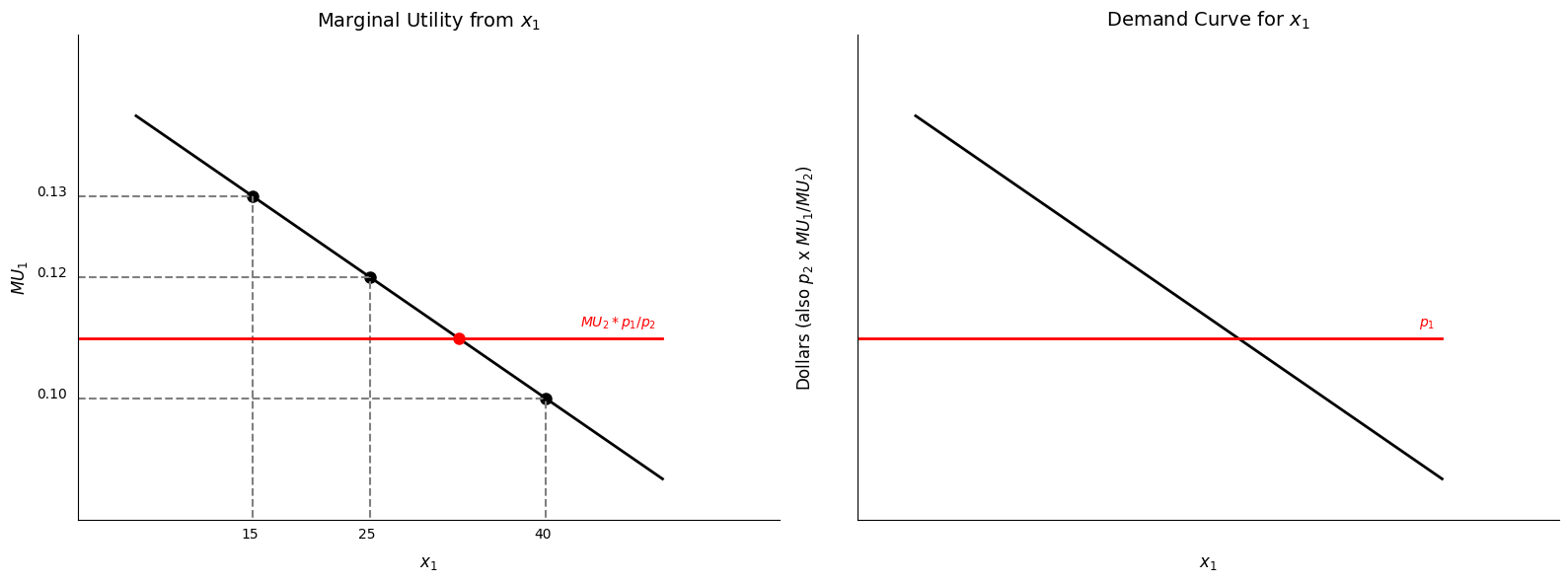
Now this is starting to look like a demand curve. Except that the y axis is not price or dollars, as you might expect, but marginal utility from apples. But in the figure below, we will fix that. In the top plot of that figure, we reproduce the bottom, marginal utility plot from the figure above, with a twist.
Specifically, we indicate how many apples the consumer will choose along her marginal utility curve. How do we figure that out? Well, we consider the benefits and costs of an extra apple. The benefit of an extra apple is the marginal utility from that apple, which is measured on the y-axis. The cost of an apple is the incremental utility from the books that the consumer has to give up to get an extra apple. If the marginal benefit of an apple is bigger than the marginal cost in terms of lost utility from books, then the consumer will consume one more apple. If the incremental benefit of an apple is lower than the marginal cost in terms of lost utility from books, then she will not consume one more apple. By deduction, that means the consumer stops consuming more apples when the marginal benefit is equal to the marginal cost. We indicate this with x1*.
But how do we derive the marginal cost from consuming one more apple? How much incremental utility from books does that cost? Recall that the consumer has a budget constraint. And the relative price of apples to books (the slope of the budget line) tells you how many books the consumer gives up for each apple she consumes. If we multiply that by the marginal utility of books (MU2), we get the marginal utility from books lost when the consumer purchases one more apple. So the consumer stops consuming more apples when the marginal utility of apples, MU1, is equal to the number of books you have to give up for that apple times the marginal utility of books, (p1/p2) x MU2.
The bottom plot gives our demand curve. The demand curve has the price of apples on the y axis. To obtain that, you just have to multiple everything, including the y-axis in the top plot with MU1 on the y-axis, by p2/MU2. If you do this, the marginal utility (of apples) curve becomes a demand curve for apples. And the cost of apples becomes p1 (because (p1/p2) x MU2 x p2/MU2 = p1).